Lagranto
The goal of this section is show how to calculate trajectories, analyzed them and plot them using the lagranto package.
Calculation
The lagranto package provide a class, dypy.lagranto.LagrantoRun, to wrap the Lagranto programs in python. It allow to calculate trajectories in parallel. You can take a look at the docstring to get familiar with the class.
Let’s say that we want to calculate Warm Conveyor Belt trajectories for a 5 day period in June 2013.
Using Era-Interim we can start trajectories every 6 hour and we will calculate them for 48 hours forward in time. Since dypy.lagranto.LagrantoRun needs a list of (startdate, enddate), we can build the dates as follow:
from datetime import datetime, timedelta
from dypy.small_tools import interval
startdate = datetime(2013, 6, 1, 0)
enddate = startdate + timedelta(days=5)
dates = [(d, d + timedelta(hours=48)) for d in
          interval(startdate, enddate, timedelta(hours=6))]
If the Era-interim data are in the erainterim folder and if the output files should be written in the output folder, then the dypy.lagranto.LagrantoRun can be initialized as follow:
from dypy.lagranto import LagrantoRun
lrun = LagrantoRun(dates, workingdir='erainterim',
                   outputdir='output', version='ecmwf')
We want to start the trajectories every 20km in the box [5E, 40E, 30N, 60N], so let’s create a starting file:
specifier = "'box.eqd(5,20,40,50,20)@profile(850,500,10)@hPa'"
out_create_startf = lrun.create_startf(startdate, specifier, tolist=True)
The tolist argument is needed if we want to use the same staring file for all starting time of the trajectories. We can now calculate the trajectories, but first starting for a single date to test our setup:
out_caltra = lrun.caltra(*dates[1])
We can also test tracing Q along a trajectories:
out_trace = lrun.trace(dates[1][0], field='Q 1.')
We can now calculate and trace the trajectories in parallel, but for this we will use a tracevars file:
tracevars = """Q         1.    0 P
U          1.    0 P
"""
out = lrun.run_parallel(trace_kw={'tracevars_content': tracevars}, type='both')
The tracevars_content keyword argument will be passed to trace to create a tracevars file with Q and U. The type keyword argument determine what is run in parallel, currently both, trace, and caltra are available.
Analyze
Now that we have calculated trajectories let’s read them and analyze them. By default the name of the files are formatted as lsl_{:%Y%m%d%H}.4. So if we want to read the trajectories started at 00 UTC 01 June 2013 we can do as follow:
from dypy.lagranto import Tra
filename_template = 'output/lsl_{:%Y%m%d%H}.4'
filename = filename_template.format(date=dates[-1][0])
trajs = Tra()
trajs.load_netcdf(filename)
print(trajs)
We can now test if the trajectories fulfill the standard criteria for WCB, an ascent greater than 500 hPa in 48 hours. To make it clear, the goal of this exmple is not to replace the fortran routines of the LAGRANTO package but to illustrate the possibilities that python provides to analyze trajectories using a simple example.
wcb_index = np.where((trajs['p'][:, :1] - trajs['p']) > 500)
wcb_trajs = Tra()
wcb_trajs.set_array(trajs[wcb_index[0], :])
print(wcb_trajs)
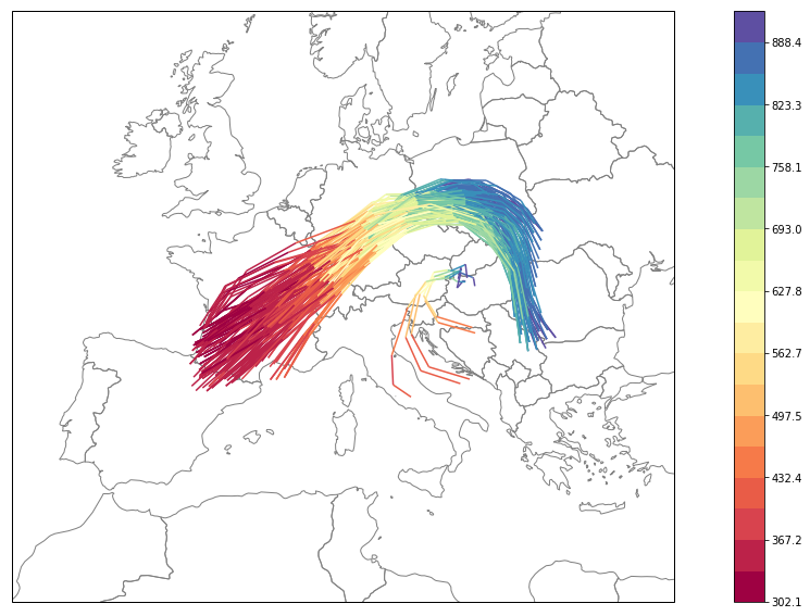
Plotting
Now that we have WCB trajectories, let’s plot them on a map. We will use cartopy for this.
import cartopy.crs as ccrs
import cartopy.feature as cfeature
from dypy.plotting import plot_trajs
import matplotlib.pyplot as plt

crs = ccrs.Stereographic(central_longitude=180 - 170,
                         central_latitude=90 - 43,
                         true_scale_latitude=90 - 43)
fig = plt.figure()
ax = plt.axes(projection=crs)
land_50m = cfeature.NaturalEarthFeature('cultural', 'admin_0_countries',
                                         '50m', edgecolor='gray',
                                         facecolor='none', linewidth=0)
ax.add_feature(land_50m)
ax.set_extent([-10, 28, 30, 60])
plot_trajs(ax, wcb_trajs, 'p')
# fig.savefig('wcb_trajs_{date:%Y%m%d_%H}.pdf'.format(date=dates[-1][0]), bbox_inches='tight')
Writing
The WCB trajectories can also be written to disk as follow:
wcb_trajs.write_netcdf('output/wcb_trajs.nc')